Graffiti - a Python library for declarative computation

Today I’m very excited to announce the release of graffiti, a Python library for declarative graph computation. To get going with graffiti, you can either install from PyPI via pip or checkout the source and install it directly:

# via pip install
pip install graffiti

# via github
git clone https://github.com/SegFaultAX/graffiti.git
cd graffiti/
python setup.py install

If you’d like to jump right in, the README has a brief introduction and tutorial. Also check out Prismatic’s Plumbing library which served as a huge source of inspiration for graffiti.

the problem

Consider the following probably entirely reasonable Python snippet:

def stats(xs):
  n = len(xs)
  m = float(sum(xs)) / n
  m2 = float(sum(x ** 2 for x in xs)) / n
  v = m2 - m ** 2

  return {
    "xs": xs,
    "n": n,
    "m": m,
    "m2": m2,
    "v": v,
  }

print stats(range(10))
#=> {'v': 8.25, 'xs': [0, 1, 2, 3, 4, 5, 6, 7, 8, 9], 'm2': 28.5, 'm': 4.5, 'n': 10}

This somewhat contrived example demonstrates two interesting ideas. First, it’s very common to build a computational “pipeline” by starting with some initial value (xs above) and pass it through a series of transformations to reach our desired result. Second, the intermediate values of that pipeline are often useful in their own right, even if they aren’t necessarily what we’re trying to calculate right now. Unfortunately the above example breaks down in a couple of key aspects, so let’s examine each of them in turn. Afterwards, I’ll show how to represent the above pipeline using graffiti and discuss how some of these pitfalls can be avoided.

One function to rule them all

The first obvious issue with our stats function is it’s doing everything. This might be perfectly reasonable and easy to understand when the number of things it’s doing is small and well-defined, but as the requirements change, this function will likely become increasingly brittle. As a first step, we might refactor the above code into the following smaller functions:

def mean(xs):
  return float(sum(xs)) / len(xs)

def mean_squared(xs):
  return float(sum(x ** 2 for x in xs)) / len(xs)

def variance(xs):
  return mean_squared(xs) - mean(xs) ** 2

def stats_redux(xs):
  return {
    "xs": xs,
    "m": mean(xs),
    "m2": mean_squared(xs),
    "v": variance(xs),
  }

Is this code an improvement over the original? On the one hand, we’ve pulled out a bunch of useful functions which we can reuse elsewhere, so that’s an obvious +1 for reusability. On the other hand, the stats_redux function is still singularly responsible for assembling the results of the other stats functions, making it into something of a “god function”. Furthermore, consider how many times sum and len are being called compared to the previous implementation. With the functions broken apart, we’ve lost the benefit of local reuse of those intermediate computations. For simple examples like the one above, this might be a worthwhile trade-off, but in a real application there could be vastly more time consuming operations where it would be useful to build on the intermediate results.

It’s also worth considering that in a more complex example the smaller functions might have more complex arguments putting a higher burden on the caller. For this reason it’s convenient to have a single (or small group of) functions like stats_redux to properly encode those constraints.

Eager vs. lazy evaluation

Another significant issue with the original stats function is the eagerness with which it evaluates. In other words, there isn’t an obvious way to compute only some of the keys. The simplest way to solve this problem is to break down the function as we did in the previous section, and then only manually compute the exact values as we need them. However, this solution comes with the same set of caveats as before:

We lose local reuse of [potentially expensive to compute] intermediate values.
It puts more burden on the user of the library, since they have to know and understand how to utilize the utility functions.

One possible approach to solving this problem is to manually encode the dependencies between the nodes to make it easier for the caller, but also allowing parts of the pipeline to be applied lazily:

def mean(xs):
  n = len(xs)
  return { "n": n, "m": float(sum(xs)) / n, "xs": xs }

def mean_squared(xs):
  md = mean(xs)
  md["m2"] = float(sum(x ** 2 for x in xs)) / md["n"]
  return md

def variance(xs):
  m2d = mean_squared(xs)
  m2d["v"] = m2d["m2"] - m2d["m"] ** 2
  return m2d

xs = range(10)
mean(xs)
#=> {'xs': [0, 1, 2, 3, 4, 5, 6, 7, 8, 9], 'm': 4.5, 'n': 10}
mean_squared(xs)
#=> {'xs': [0, 1, 2, 3, 4, 5, 6, 7, 8, 9], 'm2': 28.5, 'm': 4.5, 'n': 10}
variance(xs)
#=> {'v': 8.25, 'xs': [0, 1, 2, 3, 4, 5, 6, 7, 8, 9], 'm2': 28.5, 'm': 4.5, 'n': 10}

The above code might seem silly (because it is), but it solves the problem of eagerness by breaking the computation down into steps that build on eachother linearly. We also get reuse of intermediate values (such as len) essentially for free. The biggest issues with this approach are:

It basically doesn’t work at all if the computational pipeline isn’t perfectly linear.
It might require the caller to have some knowledge of the dependency graph.
It doesn’t scale in general to things of arbitrary complexity.
The steps aren’t as independently useful as they were in the previous section due to the incredibly high coupling between them.

When the source ain’t enough

The final issue I want to discuss with our (now beaten-down) stats function is that of transparency. In simple terms, it is extremely difficult to understand how xs is being threaded through the pipeline to arrive at a final result. From an outside perspective, we see data go in and we see new data come out, but we completely miss the relationships between those values. As our application grows in complexity (and it will), being able to easily visualize and reason about the interdependencies of each component becomes extraordinarily important. Unfortunately, all of that dependency information is hidden away inside the body of the function, which means we either have to rely on documentation (damned lies) or we have to read the source. Furthermore, reading the source is rarely the most efficient way to quickly get an intuition about what the code is actually trying to do.

Complexity [in software systems] grows at least as fast as the square of the size of the program

- Gerald Weinberg, Quality Software Management: Systems Thinking

In my experience, there isn’t a good general solution to this problem. Some applications reify certain kinds of dependencies in the type system. Others will use patterns like Dependency Injection or Inversion of Control to push dependency information into the application configuration or framework container. However, as the application tends towards complexity, these solutions can become just as brittle or pathologically difficult to understand as their imperative counter-parts.

graffiti to the rescue!

Here’s a quick recap of the issues we’ve identified so far about stats:

It’s doing too much stuff, but we’d like to have a single (or small number) of functions responsible for building the results we want.
It eagerly evaluates all of its results, but we’d like to be able to ask for some subset of those keys.
It’s hard to see how the final dictionary/map is being generated and, in particular, what the dependencies between the different values are.
Pulling it all apart has potential performance implications if intermediate values are computed multiple times.

Let’s rewrite stats to use graffiti:

from graffiti import Graph

stats_desc = {
  "n": lambda xs: len(xs),
  "m": lambda xs, n: float(sum(xs)) / n,
  "m2": lambda xs, n: float(sum(x ** 2 for x in xs)) / n,
  "v": lambda m, m2: m2 - m ** 2
}

graph = Graph(stats_desc)
graph(xs=range(10))
#=> {'v': 8.25, 'xs': [0, 1, 2, 3, 4, 5, 6, 7, 8, 9], 'm2': 28.5, 'm': 4.5, 'n': 10}

So what’s going on here? stats_desc is a “graph descriptor”, or in other words a description of the fundamental aspects of our computational pipeline. The Graph class accepts one of these descriptors (which is just a simple dict/map), and compiles it into a single function that accepts as arguments the root inputs (xs in this case), and then builds the rest of the graph according to the specification.

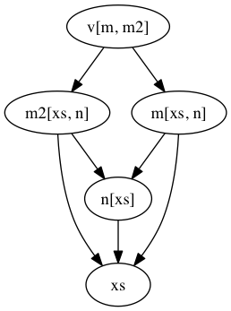
Ok, so this just seems like an obtuse way to represent the stats function. But because we’ve represented the pipeline as a graph, graffiti can do some incredibly useful operations. For example, you can visualize the graph:

# requires pydot: pip install pydot
graph.visualize()

Or we can ask it to partially evaluate the graph for only some of its keys:

graph(xs=range(10), _keys={"m2"})
#=> {'xs': [0, 1, 2, 3, 4, 5, 6, 7, 8, 9], 'm2': 28.5, 'n': 10}

We can even resume a previously partially computed graph:

prev = {'xs': [0, 1, 2, 3, 4, 5, 6, 7, 8, 9], 'm2': 28.5, 'n': 10}
graph(prev)
#=> {'v': 8.25, 'xs': [0, 1, 2, 3, 4, 5, 6, 7, 8, 9], 'm2': 28.5, 'm': 4.5, 'n': 10}

Graphs can be nested arbitrarily, provided there are no dependency cycles:

from collections import Counter

stats_desc = {
  "n": lambda xs: len(xs),
  "m": lambda xs, n: float(sum(xs)) / n,
  "m2": lambda xs, n: float(sum(x ** 2 for x in xs)) / n,
  "v": lambda m, m2: m2 - m ** 2,
  "avg": {
    "sorted": lambda xs: sorted(xs),
    "median": lambda sorted, n: sorted[n/2],
    "mode": lambda xs: Counter(xs).most_common()[0][0]
  }
}

graph = Graph(stats_desc)
graph(xs=[1, 2, 2, 3, 3, 3, 4, 4, 4, 4][::-1])
# {'avg': {'median': 3, 'mode': 4, 'sorted': [1, 2, 2, 3, 3, 3, 4, 4, 4, 4]},
#  'm': 3.0,
#  'm2': 10.0,
#  'n': 10,
#  'v': 1.0,
#  'xs': [4, 4, 4, 4, 3, 3, 3, 2, 2, 1]}

Graph descriptors are just normal dicts/maps, so non-dict/non-function values work normally:

desc = {
  "a": "Hello, world!",
  "b": [1, 2, 3, 4],
  "c": {"foo", "bar", "baz"}
}

graph = Graph(desc)
graph()
#=> {'a': 'Hello, world!', 'c': set(['bar', 'foo', 'baz']), 'b': [1, 2, 3, 4]}

Graphs can accept optional arguments:

desc = {
  "a": lambda xs, m=2: [x * m for x in xs]
}

graph = Graph(desc)
graph(xs=range(5))
#=> {'a': [0, 2, 4, 6, 8], 'xs': [0, 1, 2, 3, 4]}

graph(xs=range(5), m=10)
#=> {'a': [0, 10, 20, 30, 40], 'xs': [0, 1, 2, 3, 4], 'm': 10}

Lambdas in Python are quite limited as they are restricted to a single expression. Graffiti supports a decorator-based syntax to help ease the creation of more complex graphs:

graph = Graph()

@graph.node("len")
def length(xs):
  return len(xs)

@graph.node
def mean(xs, len):
  return float(sum(xs)) / len

graph.add_node("sorted", lambda xs: sorted(xs))

sub = graph.subgraph("avg")

@sub.node
def median(sorted, len):
  return sorted[len / 2]

graph(xs=range(10))
# {'avg': {'median': 5},
#  'len': 10,
#  'mean': 4.5,
#  'sorted': [0, 1, 2, 3, 4, 5, 6, 7, 8, 9],
#  'xs': [0, 1, 2, 3, 4, 5, 6, 7, 8, 9]}

graph.graph
# {'avg': <graffiti.Graph object at 0x101e96e50>,
#  'len': <function length at 0x101e996e0>,
#  'mean': <function mean at 0x101e998c0>,
#  'sorted': <function <lambda> at 0x101e99848>}

So how does this stack up to our stats function?

Too much stuff –> each node is responsible for one aspect of the overall computational graph.
Eager evaluation –> graffiti can partially apply as much of the graph as necessary, and you can incrementally resume a graph as more values are required.
Hard to see dependencies –> graffiti’s powerful visualization tools give you an amazingly useful way to help gain an intuition about how data flows through the pipeline. Moreover, since the graph is just a dict, it’s easy to inspect it, play with it at the repl, build it up iteratively or across multiple files/namespaces, etc.
Performance penalties from decoupling –> everything stays decoupled and intermediate values are shared throughout the graph. graffiti knows when not to evaluate keys if it already has done previously making graphs trivially resumable (see #2).

Hopefully some of these examples have demonstrated the power graffiti gives you over your computational pipeline. Importantly, since graph descriptors are just data (and the Graph class itself is just a wrapper around that data), you can do the same fundamental higher-order operations on them that you can normal dictionaries. And I’ve just started scratching the surface of what graffiti can do!

If you’re interested in helping out, send me a note SegFaultAX on Twitter and Github.

Macroexpand the Mind

Graffiti - a Python Library for Declarative Computation

the problem

One function to rule them all

Eager vs. lazy evaluation

When the source ain’t enough

graffiti to the rescue!

Comments